Time Series Forecasting
Time-series forecasting project comparing Statistical Models (ARIMAX) and Machine Learning for soil water content prediction.
Predicting soil moisture is inherently a time-series problem: today’s water content depends on yesterday’s, modulated by external factors like rainfall and evapotranspiration. In this project, I modeled these temporal dynamics using Statistical Time Series methods (ARIMAX, Panel Data) and compared them against Machine Learning regressors.
Objectives
- Analyze the temporal structure of soil moisture data (Stationarity, Seasonality, Autocorrelation).
- Develop an ARIMAX model and panel data models to forecast soil moisture using weather variables as exogenous inputs.
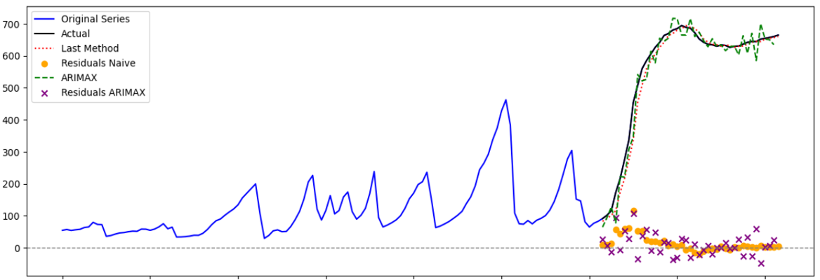
- Benchmark the statistical approach against ML models (Naive, Random Forest, SVR, XGBoost) to evaluate performance.
My role
- Conducted stationarity tests (ADF) and decomposition analysis.
- Tuned ARIMA hyperparameters (
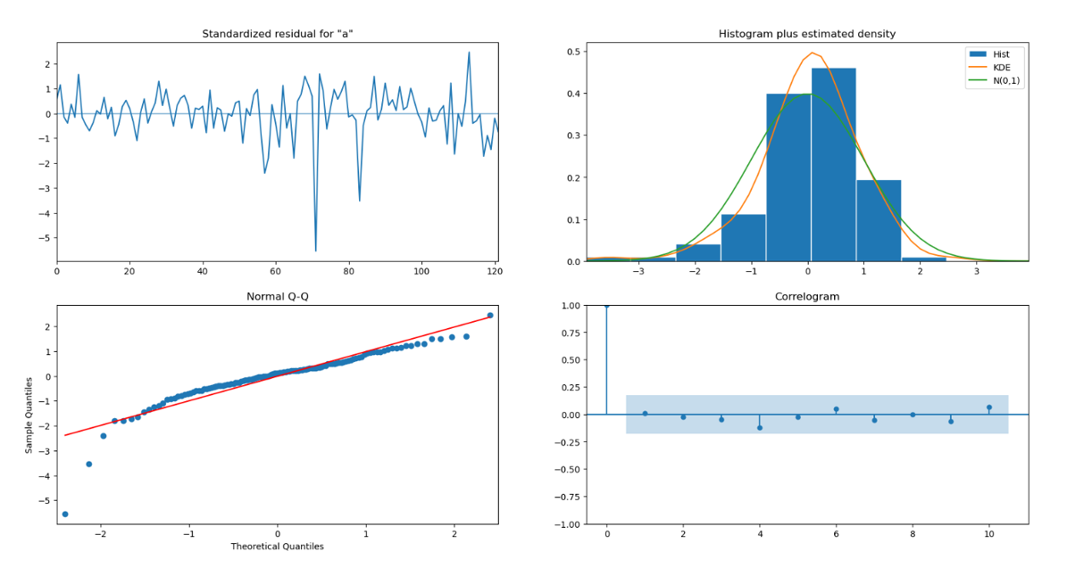
p,d,q) using ACF/PACF plots. - Evaluated panel data models to capture multi-site soil moisture dynamics.
- Engineered lag and rolling window features for ML baselines.
- Compared models using time-aware cross-validation metrics.
Tech Stack
| Language | Python 3.8+ |
|---|---|
| Statistics | Statsmodels (ARIMA/SARIMAX), Panel Data Models |
| ML | Scikit-Learn (Random Forest, SVR, XGBoost) |
| Viz | Matplotlib, Seaborn |
Repository Structure
The project separates statistical modeling from ML pipelines:
01_EDA_Time_SeriesStationarity & Decomposition02_ARIMAX_ImplementationStatistical Modeling03_Panel_Data_ModelsMulti-site temporal modeling04_ML_ComparisonRandom Forest/SVR BaselinesdocsLiterature review & approach
The Challenge: Autocorrelation and External Forcing
Soil moisture data presents a dual challenge:
- Strong Autocorrelation: The value at time t is highly correlated with t-1.
- External Forcing: Changes are driven by external “shocks” (Rainfall, Evapotranspiration).
Standard ML models struggle with raw temporal dependencies unless engineered lag features are included. ARIMAX explicitly models the autoregressive structure, while Panel Data models capture multi-site dependencies and site-specific heterogeneity.

Methodology: Statistical vs. ML
The workflow was designed to rigorously test the statistical properties of the data before modeling.
- Stationarity Analysis: Used the Augmented Dickey-Fuller (ADF) test to check for unit roots. The series required differencing ($d=1$) to become stationary.
- Order Selection: Analyzed ACF (Autocorrelation) and PACF (Partial Autocorrelation) plots to determine the initial
p(AR) andq(MA) terms for the ARIMA model. - ARIMAX Modeling: Implemented the model using
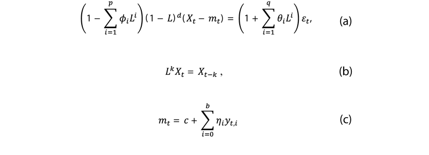
statsmodels. Rainfall and Temperature were fed as exogenous variables to help the model react to weather events. - ML Benchmarking: Trained Random Forest and SVR models. To make the comparison fair, the ML dataset was augmented with “Lag Features” (shifting the target column) to simulate the memory effect inherent in ARIMA.


Results: Interpretability vs. Precision
The analysis provided clear distinctions between the two approaches:
- ARIMAX (Statistical): Provided excellent interpretability. The model coefficients allowed for quantifying exactly how much a mm of rain impacts soil moisture over time. However, it struggled with the non-linear “drying phases” of the soil.
- Panel Data Models: Captured site-specific heterogeneity, improving reliability across multiple locations.
- Machine Learning (RF): Outperformed ARIMAX in terms of raw RMSE (Root Mean Square Error), particularly in capturing non-linear relationships during long dry spells.
The project concluded that while ML offers higher raw accuracy, ARIMAX and Panel Data models provide a more robust framework for understanding the causal relationship between weather inputs and soil dynamics.

Note: To maintain confidentiality, all company names, locations, dates, and specific proprietary values have been anonymized or modified. The analysis focuses on the technical methodology and challenges encountered during the project.