Spatial Interpolation
Comparative analysis of geostatistical algorithms to transform sparse sensor data into continuous surface maps.
In environmental monitoring, data is often limited to specific point locations. This project addresses the “missing data” problem by comparing deterministic and geostatistical algorithms to generate continuous high-resolution maps from sparse inputs.
Objectives
- Transform discrete point data from sensors into continuous spatial surfaces.
- Benchmark IDW (Inverse Distance Weighting) against Ordinary Kriging.
My role
- Processed geospatial vector data (Shapefiles) and sensor readings.
- Implemented interpolation algorithms using Python libraries.
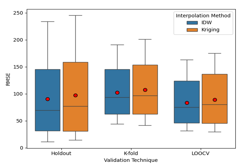
- Validated model accuracy using Cross-Validation (RMSE metrics).
Tech Stack
| Language | Python 3.9+ |
|---|---|
| Geospatial | PyKrige, SciPy |
| Viz | Matplotlib |
| DevOps | uv (package manager), Jupyter |
Repository Structure
dataRaw Shapefiles & CSVsimagesStores generated plots and visualizationsnotebooksExploratory data analysis and statistical testingscriptsFor generating comparisons and descriptive statisticspackageCore package containing the implementation of interpolation algorithms
The Challenge: From Points to Surfaces
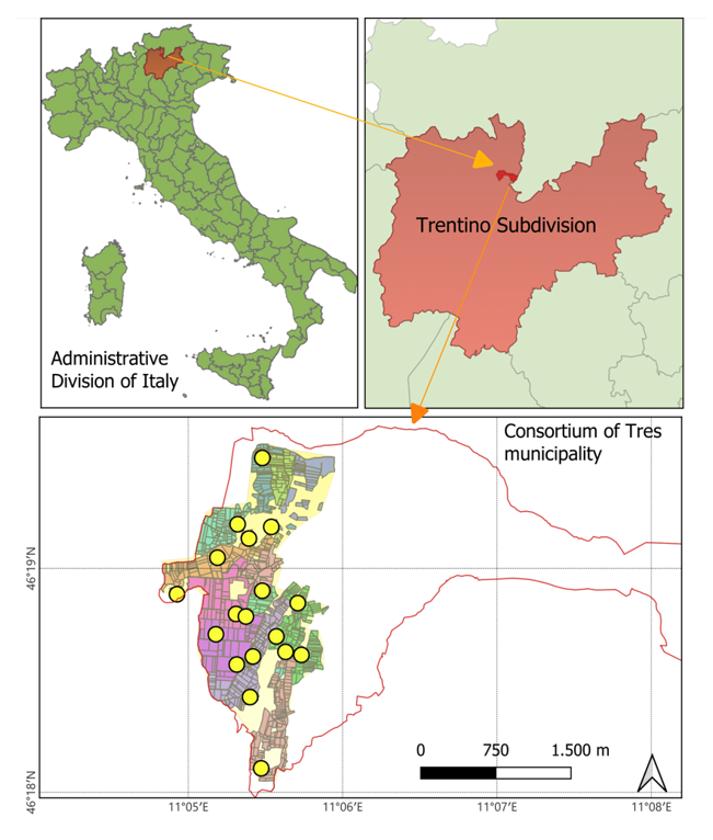
The core task was to estimate temperature and precipitation values for locations where no sensors existed. The input dataset consisted of scattered weather stations across a region in Northern Italy.
- Input: Discrete coordinates (Lat, Lon) with value $Z$ (e.g., Temperature).
- Output: A continuous raster grid (heatmap) covering the entire area.

Methodology & Results
I compared three approaches to fill the spatial gaps:
- IDW: Fast but sensitive to outliers, creating “bullseye” artifacts.
- RBF: Smooth mathematical surface fitting.
- Ordinary Kriging: A geostatistical method that minimizes error variance by modeling spatial autocorrelation (Variogram).
The Verdict: Validation showed that Kriging provided the most realistic representation of environmental phenomena, minimizing the Root Mean Square Error (RMSE) compared to the deterministic methods.

Full Documentation
The methodological details, mathematical formulations of the spatial error models, and complete variable analysis are presented in the associated academic paper referenced below:
Read Full Paper View Presentation Slides