Pandas

Pandas#

Pandas is a powerful Python library for data manipulation and analysis. It provides data structures and functions to efficiently work with structured data, such as tabular data and time series. Pandas introduces two primary data structures, namely Series and DataFrame, which allow for easy indexing, slicing, filtering, and transformation of data. With Pandas, you can handle missing data, perform statistical calculations, apply data reshaping operations, and visualize data. It also integrates well with other libraries, such as NumPy and Matplotlib, making it a popular choice for data analysis tasks, data cleaning, preprocessing, and exploratory data analysis (EDA).

import pandas as pd

Series#

Creation#

sr = pd.Series(data = [10, 20, 30], name = 'sum_10')  # simple creation with name
sr

  10
  20
  30
Name: sum_10, dtype: int64

sr2 = pd.Series(data = [10, 20, 30],  # creation with indexes
          index = ['a', 'b', 'c'])
sr2

a    10
b    20
c    30
dtype: int64

sr3 = pd.Series(data = {'a': 10, 'b': 20, 'c': 30})  # creation from dictionary
sr3

a    10
b    20
c    30
dtype: int64

name: returns the name of the series
rename: changes the name
dtype: returns the type of the elements in the series
index: returns the indexes of the series
to_numpy: access data underlying the array

print(sr.name)
print(sr.rename('sum'))
print(sr.dtype)
print(sr.index)
print(sr.to_numpy())

sum_10
0    10
1    20
2    30
Name: sum, dtype: int64
int64
RangeIndex(start=0, stop=3, step=1)
[10 20 30]

Access, Operations, Functions#

Just as Numpy’s arrays

Series of Strings Methods#

Method	Paramethers	Description
`str.cat`	others=None, sep=None	Concatenates strings in the series with given separator
`str.split`	pat*=None, n=-1	Splits strings in the series around given separator from the beginning
`str.rsplit`	pat*=None, n=-1	Splits strings in the series around given separator from the end
`str.get`	i	Extracts element from each component at specified position in the series
`str.join`	sep	Joins lists contained as elements in the series with passed delimiter
`str.get_dummies`	sep*=’	‘
`str.contains`	pat, regex*=True	Returns boolean series if each string contains pattern/regex
`str.replace`	pat, repl, n=-1, regex*=True	Replaces occurrences of pattern/regex with some other string or the return value of a callable given the occurrence

Others as python-basics: str.capitalize, str.casefold, str.lower, str.upper, str.len, …

Dataframe#

Creation#

df = pd.DataFrame([[1, 2, 3],  # simple dataframe creation (from lists)
              [4, 5, 6],
              [7, 8, 9]])

df = pd.DataFrame([[1, 2, 3],  # creation with indexes and colunms names
              [4, 5, 6],
              [7, 8, 9]],
             index = ['R1', 'R2', 'R3'],
             columns = ['C1', 'C2', 'C3'])

Creation from a Support

Support	Example
Array	`pd.DataFrame(np.array([['Tom', 7], ['Mike', 15], ['Tiffany', 3]]))`
Dictionary	`pd.DataFrame({'Name': ['Tom', 'Mike', 'Tiffany'], 'Number': [7, 15, 3]})`
List	`pd.DataFrame([['Tom', 7], ['Mike', 15], ['Tiffany', 3]])`
List of Dictionaries	`pd.DataFrame({'Name': 'Tom', 'Number': 7}, {'Name': 'Mike', 'Number': 15}, {'Name': 'Tiffany', 'Number': 3}`
Series	`pd.DataFrame({'Name': pd.Series(['Tom', 'Mike', 'Tiffany']), 'Number': pd.Series([7, 15, 3])})`
Tuple	`pd.DataFrame(zip(['Tom', 'Mike', 'Tiffany'], [7, 15, 3]))`

Creation from File

File	Function
CSV	`read_csv`
Excel	`read_excel`
Html	`read_html`
Json	`read_json`
Text	`read_csv` with `delimiter='\t'`

Access#

Indexing with []

df['C1']  # returns a series from a column

R1    1
R2    4
R3    7
Name: C1, dtype: int64

df[['C1']]  # returns a dataframe from a column

# df[0:1]  returns a dataframe from a row

	C1
R1	1
R2	4
R3	7

df[['C1', 'C2']]  # returns a dataframe with multiple columns

# df[0:2]  returns a dataframe with multiple rows

	C1	C2
R1	1	2
R2	4	5
R3	7	8

Boolean indexing

Boolean indexing in Pandas is a technique where you filter rows from a DataFrame by using a series of boolean values. Each boolean value indicates whether a specific condition is met for its corresponding row. By applying this boolean series as an index to the DataFrame, you retrieve only the rows that fulfill the condition. It’s a convenient method for extracting subsets of data that adhere to specific logical requirements.

df[df['C1'] > 1]

	C1	C2	C3
R2	4	5	6
R3	7	8	9

It returns an Object for single selection, Series for one row/column, otherwise DataFrame

loc method

Using the loc function in Pandas involves selecting data from a DataFrame based on label-based indexing. You specify row and column labels to access specific data points. This method is particularly useful when you want to work with data using its meaningful labels rather than numeric positions. It provides a convenient way to extract data based on labels, enhancing readability and understanding.

df.loc[['R1', 'R2'], ['C1']]

	C1
R1	1
R2	4

It returns an Object for single selection, Series for one row/column, otherwise DataFrame

iloc method

Using iloc in Pandas means selecting data from a DataFrame by specifying integer-based row and column indices. This approach lets you retrieve data using numerical positions, offering a precise way to extract information from specific locations within the DataFrame. It’s particularly useful for numeric-oriented data retrieval tasks.

df.iloc[[0, 1], [0]]

	C1
R1	1
R2	4

It returns an Object for single selection, Series for one row/column, otherwise DataFrame

query method

The query function in Pandas allows you to filter a DataFrame by providing a string expression that represents a condition. This expression is evaluated to produce a boolean series that identifies rows matching the condition. This function simplifies the process of filtering data based on specific criteria, making the code more concise and readable. It’s a helpful tool for selecting rows that meet certain conditions in a more intuitive and SQL-like manner.

df.query('C1 > 1 & C2 == 5')

	C1	C2	C3
R2	4	5	6

It returns an Object for single selection, Series for one row/column, otherwise DataFrame

Inspection#

df = pd.read_csv('cycling_data.csv')

head: returns the firsts n rows (default = 5) of the dataframe
tail: returns the lasts n rows (default = 5) of the dataframe
shape: returns the shape of the dataframe
dtypes: returns the type of the elements in the dataframe
info: returns information about the dataframe itself, such as dtypes, memory usages and non-null values
describe: provides summary statistics of the values within a dataframe

Examples:

df.head(10)  # shows the firsts 10 rows

	Date	Name	Type	Time	Distance	Comments
0	10 Sep 2019, 00:13:04	Afternoon Ride	Ride	2084	12.62	Rain
1	10 Sep 2019, 13:52:18	Morning Ride	Ride	2531	13.03	rain
2	11 Sep 2019, 00:23:50	Afternoon Ride	Ride	1863	12.52	Wet road but nice weather
3	11 Sep 2019, 14:06:19	Morning Ride	Ride	2192	12.84	Stopped for photo of sunrise
4	12 Sep 2019, 00:28:05	Afternoon Ride	Ride	1891	12.48	Tired by the end of the week
5	16 Sep 2019, 13:57:48	Morning Ride	Ride	2272	12.45	Rested after the weekend!
6	17 Sep 2019, 00:15:47	Afternoon Ride	Ride	1973	12.45	Legs feeling strong!
7	17 Sep 2019, 13:43:34	Morning Ride	Ride	2285	12.60	Raining
8	18 Sep 2019, 13:49:53	Morning Ride	Ride	2903	14.57	Raining today
9	18 Sep 2019, 00:15:52	Afternoon Ride	Ride	2101	12.48	Pumped up tires

df.tail(10)  # shows the lasts 10 rows

	Date	Name	Type	Time	Distance	Comments
23	1 Oct 2019, 13:45:55	Morning Ride	Ride	2222	12.82	Beautiful morning! Feeling fit
24	2 Oct 2019, 00:13:09	Afternoon Ride	Ride	1756	NaN	A little tired today but good weather
25	2 Oct 2019, 13:46:06	Morning Ride	Ride	2134	13.06	Bit tired today but good weather
26	3 Oct 2019, 00:45:22	Afternoon Ride	Ride	1724	12.52	Feeling good
27	3 Oct 2019, 13:47:36	Morning Ride	Ride	2182	12.68	Wet road
28	4 Oct 2019, 01:08:08	Afternoon Ride	Ride	1870	12.63	Very tired, riding into the wind
29	9 Oct 2019, 13:55:40	Morning Ride	Ride	2149	12.70	Really cold! But feeling good
30	10 Oct 2019, 00:10:31	Afternoon Ride	Ride	1841	12.59	Feeling good after a holiday break!
31	10 Oct 2019, 13:47:14	Morning Ride	Ride	2463	12.79	Stopped for photo of sunrise
32	11 Oct 2019, 00:16:57	Afternoon Ride	Ride	1843	11.79	Bike feeling tight, needs an oil and pump

df.shape  # shape[0] are rows, shape[1] are columns

(33, 6)

df.dtypes

Date         object
Name         object
Type         object
Time          int64
Distance    float64
Comments     object
dtype: object

df.info()

<class 'pandas.core.frame.DataFrame'>
RangeIndex: 33 entries, 0 to 32
Data columns (total 6 columns):
 #   Column    Non-Null Count  Dtype  
---  ------    --------------  -----  
 0   Date      33 non-null     object 
 1   Name      33 non-null     object 
 2   Type      33 non-null     object 
 3   Time      33 non-null     int64  
 4   Distance  31 non-null     float64
 5   Comments  33 non-null     object 
dtypes: float64(1), int64(1), object(4)
memory usage: 1.7+ KB

df.describe()

# df.describe(include='all')  include all the summaries

	Time	Distance
count	33.000000	31.000000
mean	3512.787879	12.667419
std	8003.309233	0.428618
min	1712.000000	11.790000
25%	1863.000000	12.480000
50%	2118.000000	12.620000
75%	2285.000000	12.750000
max	48062.000000	14.570000

View vs Copy#

A view of a DataFrame is a representation that provides access to a subset of the original data. Changes made to the view will affect the original DataFrame, as they both share the same underlying data.

A copy of a DataFrame is an independent duplicate with identical data to the original at the time of copying. Modifications to a copy do not impact the original DataFrame, and vice versa.

df_copy = df.copy()

It is important to note that accessing the dataframe via [], Boolean indexing, or query generates a copy of the original dataframe, whereas the loc and iloc functions use a view. Consequently, it is necessary to use these two functions to modify values within the original dataset.

Operations#

Rename

df = df.rename(columns={'Date': 'Datetime', 'Comments': 'Notes'})  # rename columns
# df.rename(columns={'Date': 'Datetime', 'Comments': 'Notes'}, inplace=True)  equivalent

df.head()

	Datetime	Name	Type	Time	Distance	Notes
0	10 Sep 2019, 00:13:04	Afternoon Ride	Ride	2084	12.62	Rain
1	10 Sep 2019, 13:52:18	Morning Ride	Ride	2531	13.03	rain
2	11 Sep 2019, 00:23:50	Afternoon Ride	Ride	1863	12.52	Wet road but nice weather
3	11 Sep 2019, 14:06:19	Morning Ride	Ride	2192	12.84	Stopped for photo of sunrise
4	12 Sep 2019, 00:28:05	Afternoon Ride	Ride	1891	12.48	Tired by the end of the week

df = df.rename(index={0: 'row_1', 2: 'row_3'})  # rename rows
# df.rename(index={0: 'row_1', 2: 'row_3'}, inplace=True)  equivalent

df.head()

	Datetime	Name	Type	Time	Distance	Notes
row_1	10 Sep 2019, 00:13:04	Afternoon Ride	Ride	2084	12.62	Rain
1	10 Sep 2019, 13:52:18	Morning Ride	Ride	2531	13.03	rain
row_3	11 Sep 2019, 00:23:50	Afternoon Ride	Ride	1863	12.52	Wet road but nice weather
3	11 Sep 2019, 14:06:19	Morning Ride	Ride	2192	12.84	Stopped for photo of sunrise
4	12 Sep 2019, 00:28:05	Afternoon Ride	Ride	1891	12.48	Tired by the end of the week

df = df.set_index('Datetime')
df.head()

	Name	Type	Time	Distance	Notes
Datetime
10 Sep 2019, 00:13:04	Afternoon Ride	Ride	2084	12.62	Rain
10 Sep 2019, 13:52:18	Morning Ride	Ride	2531	13.03	rain
11 Sep 2019, 00:23:50	Afternoon Ride	Ride	1863	12.52	Wet road but nice weather
11 Sep 2019, 14:06:19	Morning Ride	Ride	2192	12.84	Stopped for photo of sunrise
12 Sep 2019, 00:28:05	Afternoon Ride	Ride	1891	12.48	Tired by the end of the week

df = df.reset_index()
df.head()

	Datetime	Name	Type	Time	Distance	Notes
0	10 Sep 2019, 00:13:04	Afternoon Ride	Ride	2084	12.62	Rain
1	10 Sep 2019, 13:52:18	Morning Ride	Ride	2531	13.03	rain
2	11 Sep 2019, 00:23:50	Afternoon Ride	Ride	1863	12.52	Wet road but nice weather
3	11 Sep 2019, 14:06:19	Morning Ride	Ride	2192	12.84	Stopped for photo of sunrise
4	12 Sep 2019, 00:28:05	Afternoon Ride	Ride	1891	12.48	Tired by the end of the week

Add and Remove

This section only considers cases where only one row/column is to be added or deleted. The results can be easily generalized to the case of multiple rows or columns (see also the next section), for example, using Dataframes instead of Series.

Add Column

df['Avg Speed'] = df['Distance'] * 1000 / df['Time']  # direct method (using series)
# df['Avg Speed'] = pd.Series([6, 5, 6, ...])  example with explicit series

# Alternatives
# 1) df.loc[:, 'Avg Speed'] = df['Distance'] * 1000 / df['Time']  # loc
# 2) df.iloc[:, df.shape[1]] = df['Distance'] * 1000 / df['Time']  #iloc
#    df.columns = [*df.columns[:-1], 'Avg Speed']

df.head()

	Datetime	Name	Type	Time	Distance	Notes	Avg Speed
0	10 Sep 2019, 00:13:04	Afternoon Ride	Ride	2084	12.62	Rain	6.055662
1	10 Sep 2019, 13:52:18	Morning Ride	Ride	2531	13.03	rain	5.148163
2	11 Sep 2019, 00:23:50	Afternoon Ride	Ride	1863	12.52	Wet road but nice weather	6.720344
3	11 Sep 2019, 14:06:19	Morning Ride	Ride	2192	12.84	Stopped for photo of sunrise	5.857664
4	12 Sep 2019, 00:28:05	Afternoon Ride	Ride	1891	12.48	Tired by the end of the week	6.599683

Remove Column

df = df.drop(columns=['Avg Speed'])
df.head()

	Datetime	Name	Type	Time	Distance	Notes
0	10 Sep 2019, 00:13:04	Afternoon Ride	Ride	2084	12.62	Rain
1	10 Sep 2019, 13:52:18	Morning Ride	Ride	2531	13.03	rain
2	11 Sep 2019, 00:23:50	Afternoon Ride	Ride	1863	12.52	Wet road but nice weather
3	11 Sep 2019, 14:06:19	Morning Ride	Ride	2192	12.84	Stopped for photo of sunrise
4	12 Sep 2019, 00:28:05	Afternoon Ride	Ride	1891	12.48	Tired by the end of the week

Add Row

new_row = pd.Series(['12 Oct 2019, 00:10:57', 'Morning Ride', 'Ride',
                    2331, 12.67, 'Washed and oiled bike last night'],
                    index = df.columns)
df.loc[df.index.max() + 1] = new_row

# Alternative
# df.iloc[df.shape[0]] = new_row

df.tail()

	Datetime	Name	Type	Time	Distance	Notes
29	9 Oct 2019, 13:55:40	Morning Ride	Ride	2149	12.70	Really cold! But feeling good
30	10 Oct 2019, 00:10:31	Afternoon Ride	Ride	1841	12.59	Feeling good after a holiday break!
31	10 Oct 2019, 13:47:14	Morning Ride	Ride	2463	12.79	Stopped for photo of sunrise
32	11 Oct 2019, 00:16:57	Afternoon Ride	Ride	1843	11.79	Bike feeling tight, needs an oil and pump
33	12 Oct 2019, 00:10:57	Morning Ride	Ride	2331	12.67	Washed and oiled bike last night

Remove Row

df = df.drop(index=[30, 31, 32, 33])
# df = df.drop(index=df.index[30:])  equivalent

df.tail()

	Datetime	Name	Type	Time	Distance	Notes
25	2 Oct 2019, 13:46:06	Morning Ride	Ride	2134	13.06	Bit tired today but good weather
26	3 Oct 2019, 00:45:22	Afternoon Ride	Ride	1724	12.52	Feeling good
27	3 Oct 2019, 13:47:36	Morning Ride	Ride	2182	12.68	Wet road
28	4 Oct 2019, 01:08:08	Afternoon Ride	Ride	1870	12.63	Very tired, riding into the wind
29	9 Oct 2019, 13:55:40	Morning Ride	Ride	2149	12.70	Really cold! But feeling good

Reshape

Pivot

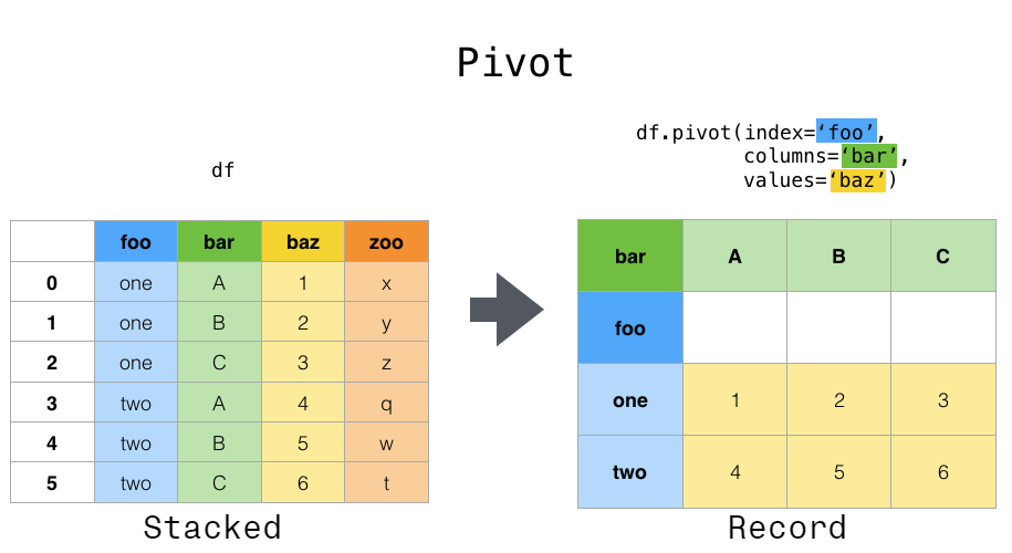
df = pd.DataFrame({'foo': ['one', 'one', 'one', 'two', 'two', 'two'],
                    'bar': ['A', 'B', 'C', 'A', 'B', 'C'],
                    'baz': [1, 2, 3, 4, 5, 6],
                    'zoo': ['x', 'y', 'z', 'q', 'w', 't']})
df.pivot(index = 'foo', columns = 'bar', values = 'baz')

bar	A	B	C
foo
one	1	2	3
two	4	5	6

Stack

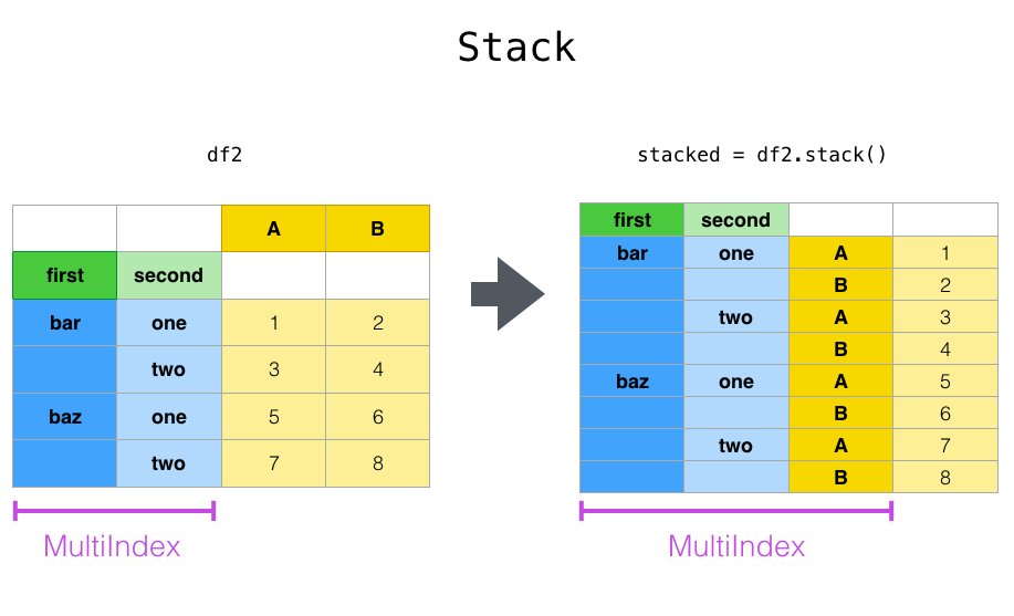
index_tuples = [('bar', 'one'), ('bar', 'two'), ('baz', 'one'), ('baz', 'two')]
multi_index = pd.MultiIndex.from_tuples(index_tuples, names=['first', 'second'])

data = {'A': [1, 3, 5, 7],
        'B': [2, 4, 6, 8]}
df2 = pd.DataFrame(data, index=multi_index)

df_stacked = df2.stack()
df_stacked

first  second   
bar    one     A    1
               B    2
       two     A    3
               B    4
baz    one     A    5
               B    6
       two     A    7
               B    8
dtype: int64

Unstack

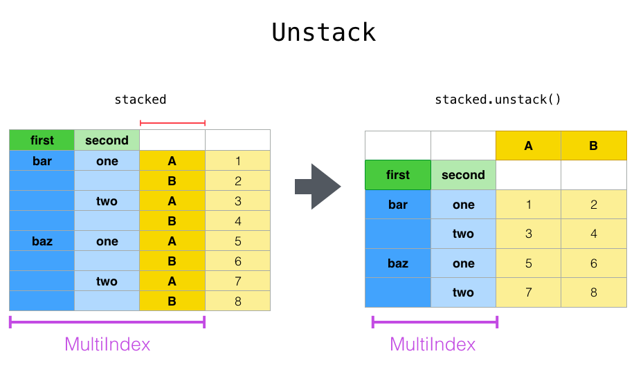
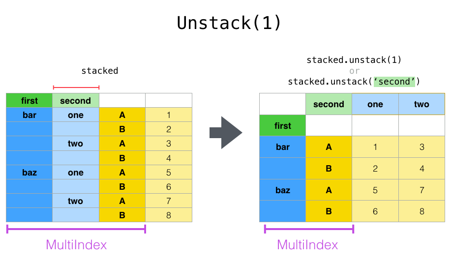
df_stacked.unstack()

# df_stacked.unstack(0)  or  df_stacked.unstack('first')
# df_stacked.unstack(1)  or  df_stacked.unstack('second')

		A	B
first	second
bar	one	1	2
bar	two	3	4
baz	one	5	6
baz	two	7	8

Melt

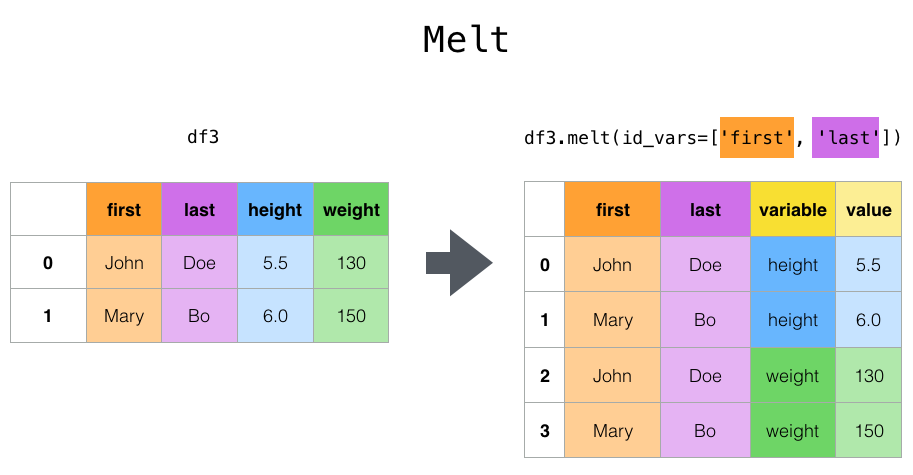
df3 = pd.DataFrame({'first': ['John', 'Mary'],
                    'last': ['Doe', 'Bo'],
                    'height': [5.5, 6.0],
                    'weight': [130, 150]})
                    
df3.melt(id_vars=['first', 'last'])

	first	last	variable	value
0	John	Doe	height	5.5
1	Mary	Bo	height	6.0
2	John	Doe	weight	130.0
3	Mary	Bo	weight	150.0

Multiple Dataframes

Concatenating two DataFrames in pandas is the process of combining them together to create a single DataFrame. This can be done either by concatenating along rows, which results in vertically stacking the DataFrames, or by concatenating along columns, which results in horizontally expanding the DataFrame. The distinction lies in whether the DataFrames are being extended vertically (rows) or horizontally (columns). The concat function in pandas is used for this operation, allowing for flexible combination of DataFrames based on the desired axis.

df1 = pd.DataFrame({'A': [1, 3, 5],
                    'B': [2, 4, 6]})
df2 = pd.DataFrame({'A': [7, 9, 11],
                    'B': [8, 10, 12]})

pd.concat((df1, df2), axis=0, ignore_index=True)  # concatenate by rows

	A	B
0	1	2
1	3	4
2	5	6
3	7	8
4	9	10
5	11	12

pd.concat((df1, df2), axis=1, ignore_index=True)  # concatenate by columns

	0	1	2	3
0	1	2	7	8
1	3	4	9	10
2	5	6	11	12

Merging two DataFrames in pandas is akin to performing SQL joins. It involves combining datasets based on common columns or indices, resulting in a unified DataFrame. The process, achieved using the merge function, is conceptually similar to SQL joins, where you define key columns for matching and specify the type of join (inner, outer, left, right) to determine how non-matching entries are handled. This enables you to consolidate data from distinct sources into a cohesive DataFrame, much like SQL joins bring together information from different database tables.

df1 = pd.DataFrame({"name": ['Magneto', 'Storm', 'Mystique', 'Batman', 'Joker', 'Catwoman', 'Hellboy'],
                    'alignment': ['bad', 'good', 'bad', 'good', 'bad', 'bad', 'good'],
                    'gender': ['male', 'female', 'female', 'male', 'male', 'female', 'male'],
                    'publisher': ['Marvel', 'Marvel', 'Marvel', 'DC', 'DC', 'DC', 'Dark Horse Comics']})
df2 = pd.DataFrame({'publisher': ['DC', 'Marvel', 'Image'],
                    'year_founded': [1934, 1939, 1992]})
                    
pd.merge(df1, df2, how='inner', on='publisher')

	name	alignment	gender	publisher	year_founded
0	Magneto	bad	male	Marvel	1939
1	Storm	good	female	Marvel	1939
2	Mystique	bad	female	Marvel	1939
3	Batman	good	male	DC	1934
4	Joker	bad	male	DC	1934
5	Catwoman	bad	female	DC	1934

Methods#

Method	Paramethers	Description
`apply`	func, axis=0	Applies a function along an axis of the dataframe
`drop_duplicates`	subset*=None, inplace=False	Returns dataFrame with duplicate rows removed
`dropna`	axis=0, subset*=None, inplace=False	Removes missing values
`duplicated`	subset*=None	Returns boolean series denoting duplicate rows
`fillna`	value=None, method=None, inplace=False	Fills na/nan values using the specified method
`groupby`	by=None	Groups dataframe using a mapper or by a series of columns
`map`	func	Apples a function to a dataframe elementwise
`sort_values`	by, axis=0, ascending=True, inplace=False	Sorts by the values along either axis

Examples

import numpy as np

df = pd.DataFrame({
  'Name': ['Alice', 'Alice', 'Alice', 'Bob', 'Bob', 'Charlie', 'David'],
  'Age': [22, 22, 22, 23, 23, 20, 19],
  'Grade': [85, 85, np.nan, 78, 69, 85, 92]})

df['Grade_sqrt'] = df['Grade'].apply(np.sqrt)
df

	Name	Age	Grade	Grade_sqrt
0	Alice	22	85.0	9.219544
1	Alice	22	85.0	9.219544
2	Alice	22	NaN	NaN
3	Bob	23	78.0	8.831761
4	Bob	23	69.0	8.306624
5	Charlie	20	85.0	9.219544
6	David	19	92.0	9.591663

age_mapping = {True: 'Young', False: 'Old'}
df['Age_category'] = df['Age'] <= 22
df['Age_category'] = df['Age_category'].map(age_mapping)
df

	Name	Age	Grade	Grade_sqrt	Age_category
0	Alice	22	85.0	9.219544	Young
1	Alice	22	85.0	9.219544	Young
2	Alice	22	NaN	NaN	Young
3	Bob	23	78.0	8.831761	Old
4	Bob	23	69.0	8.306624	Old
5	Charlie	20	85.0	9.219544	Young
6	David	19	92.0	9.591663	Young

df.sort_values(by='Age')

	Name	Age	Grade	Grade_sqrt	Age_category
6	David	19	92.0	9.591663	Young
5	Charlie	20	85.0	9.219544	Young
0	Alice	22	85.0	9.219544	Young
1	Alice	22	85.0	9.219544	Young
2	Alice	22	NaN	NaN	Young
3	Bob	23	78.0	8.831761	Old
4	Bob	23	69.0	8.306624	Old

df.groupby('Age')['Grade'].mean()

Age
19    92.0
20    85.0
22    85.0
23    73.5
Name: Grade, dtype: float64

df['Duplicated'] = df.duplicated(subset='Name')
df

	Name	Age	Grade	Grade_sqrt	Age_category	Duplicated
0	Alice	22	85.0	9.219544	Young	False
1	Alice	22	85.0	9.219544	Young	True
2	Alice	22	NaN	NaN	Young	True
3	Bob	23	78.0	8.831761	Old	False
4	Bob	23	69.0	8.306624	Old	True
5	Charlie	20	85.0	9.219544	Young	False
6	David	19	92.0	9.591663	Young	False

df.drop_duplicates(subset='Name', inplace=True)

Pandas

Contents

Pandas#

Series#

Creation#

Access, Operations, Functions#

Series of Strings Methods#

Dataframe#

Creation#

Access#

Inspection#

View vs Copy#

Operations#

Methods#